tag page

I feel lucky to have had the privilege of attending the AWS INNOVATE – AI/ML Edition Conference for the first time in my career. This conference, which was conducted on the 24th of February 2020, was not only highly informational but would very much inspire any data-driven company like Norconex to venture into performing their AI/ML projects on the cloud. The conference had sessions for users of various levels of expertise. I was hopeful that this experience would enrich my level of insight and help the team at Norconex to build our SaaS products.

AWS innovate bannerThe event kicked-off with a keynote delivered by Denis V Batalov, WW Technical Leader for AI/ML at AWS. This session showcased the application of state-of-the-art computer vision techniques and advances in machine learning and their applications in autonomous vehicles, IoT, Software development, and many more. The video clip that Batalov shared showed how they leveraged computer vision and AWS to automate their Amazon Fulfillment center seemed magical. He later moved on to shed some light on how we can use AI/ML at work and listed some of the latest AI/ML products released by AWS. The conference was planned to be conducted on various tracks which meant I had to pick and choose between numerous engaging sessions happening in parallel. Luckily, on-demand videos are made available on the AWS Innovate website which could be watched later.

Following the keynote, I jumped into the session “Prepare your Datasets at Scale using Apache Spark and SageMaker Data Wrangler.” The speaker, Chris Fregly – Developer Advocate, AI/ML at AWS, explained how we could take advantage of the distributed processing capabilities of Apache Spark using AWS SageMaker Data Wrangler. Using this combination, he illustrated how the inbuilt features of Data Wrangler empower data collection, preprocessing, and feature engineering. Fascinatingly, they have out-of-the-box components that can detect class imbalance, bias, correlation, feature importance, and many more characteristics. Using SparkML, we can train the model in parallel spark nodes and take way less time than traditional methods. At Norconex, we use AWS and Spark in our projects, and this is undoubtedly a takeaway that we could explore.

After this session, I hopped into a session by Antje Barth – Senior Developer Advocate, AI/ML at AWS on “Automating ML workflows with end-to-end pipelines.” She walked us through the ML-OPS capabilities of SageMaker Pipeline in setting up ML projects in the world of CI/CD. Another exciting part was SageMaker Model Monitor’s use to watch the model after being deployed to production. I also attended a session on AWS Security for ML by Shelbee Eigenbrode – AI/ML Specialist Solutions Architect AWS. I learned how AWS had progressed its security features in AWS transcribe to remove or protect PII data during data collection. This option could be useful for Norconex when we crawl through content involving PII data. Here is a glimpse of the AWS ML services stack which I captured in one of the sessions.

AWS ML stack

My most anticipated part of the conference was the session on “Intelligent Search” by Ryan Peterson – Enterprise Search Expert at AWS. He illustrated how Amazon Kendra, an AWS search service, houses Intelligent Search capabilities. Kendra’s core capabilities involve Natural Language Querying, Natural Language Understanding, models trained with domain-specific data, continuous improvement via user feedback, secure search (TLS and encryption), and many more. Ryan also emphasized how the workforce in various organizations wastes precious work time by looking for content and how it can be saved by using an Intelligent search. As a developer at Norconex – a pioneer in Enterprise Search, I would wholeheartedly concur. We are focused on intelligent search, which certainly offers a vast improvement over conventional search techniques.

The online/virtual conference ended with closing remarks by Chris Fregly, who provided a handy summary of the new AWS ML/AI services and their capabilities. I am happily overwhelmed by the learning experience I had at the event and eagerly look forward to participating in more quality events like this. 

This was my first year joining the open-road Elastic{ON} Tour 2019 event in Toronto on September 18, 2019. My experience at this event was fully charged with excitement from meeting with Elastic architects, operations folks, security pros, and developers alike.

The event was hosted at The Carlu in downtown Toronto. In the morning, the opening keynote was presented by Nick Drost, Senior Director of Elastic, on search solutions such as app search, site search, and enterprise search, security using SIEM, and more. One of the most exciting keynote updates was about using Elastic Cloud on Kubernetes to help simplify processes of deployment, security, scaling, upgrades, snapshots, and high availability.

The next presenter, Michael Basnight, Software Engineer at Elastic, provided an Elastic Stack roadmap with demos of the latest and upcoming features. Kibana has added new capabilities to become much more than just the main user interface of Elastic Stack, with infrastructure and logs user interface. He introduced Fleet, which provides centralized config deployment, Beats monitoring, and upgrade management. Frozen indices allows for more index storage by having indices available and not taking up HEAP memory space until the indices are requested. Also, he provided highlights on Advanced Machine Learning analytics for outlier detection, supervised model training for regression and classification, and ingest prediction processor. Elasticsearch performance has increased by employing Weak AND (also called “WAND”), providing improvements as high as 3,700% to term search and improving other query types between 28% and 292%.

Another added feature to Elasticsearch stack is advanced scoring to help boost document query, using rank_features and distance_features. The new Geo UI uses map layers.

One of the most interesting new Beats to watch for is Functionbeat, which is a serverless data shipper that can subscribe to AWS SQS event topics and CloudWatch Logs, provisions the AWS Lambda function to ship data to Elasticsearch or Elastic Cloud Enterprise.

Elastic lightweight data shippers, Beats such as Filebeat for log files, Metricbeat for metrics, Packetbeat for network data, Winlogbeat for Windows event logs, Auditbeat for audit data, Heartbeat for uptime monitoring, and the latest Functionbeat for serverless shipper can be complemented with Norconex open-source products such as Norconex HTTP Collector or Norconex Filesystem Collector to crawl meta-data from the web or filesystem, then used with the open-source Norconex Elasticsearch Committer to push data to the Elasticsearch index, directly to Elastic Cloud Enterprise or the on-prem Elasticsearch Stack. Norconex can help with collecting meta-data from enterprise web architecture or enterprise filesystems for quick searching and to get relevant results.

Packed into the morning session, Jason Rhodes, Senior Software Engineer at Elastic, presented on unified observability, combining logs, metrics, and traces.

The afternoon session, Search for All with Elastic Enterprise Search and a Site Search demo and feature walkthrough, was presented by Diane Tetrault, Director of Product Marketing at Elastic. The latest UI gives the user the ability to configure content sources they search for and connect to their own data sources. Elastic Common Schema, introduced as an open-source specification, defines a common set of document fields for data ingested into Elasticsearch (https://www.elastic.co/blog/introducing-the-elastic-common-schema).

The Security with Elastic Stack session was presented by Neil Desai, Security Specialist at Elastic. He discussed the latest security capabilities to enable analysis automation to defend from cyber threats.

The Kibana and geo update features in Canvas and Elastic Maps were presented by Raya Fratkina, Kibana Team Lead at Elastic. Learning about ways to use these functionalities makes data more actionable.

I also learned tips at Elastic Architecture at Scale, a presentation by Artem Pogossian, Solutions Architect at Elastic. He discussed scaling from local laptops to multi-clusters and cross-clusters using case deployments.

A useful new feature in machine learning and analytics was introduced by Rich Collier, Solutions Architect and ML Specialist at Elastic. He demonstrated a use case using data frames, also called transforms, a feature that allows transformation of an existing index to a secondary, summarized index. Rich showed in a demo a possible use case from a digital retailer, using time series modeling to look for anomalies and forecasting in the shopper’s purchases, integrating Canvas UI designed in Kibana to build real-time data models. It was amazing to see the ability in demo to detect possible fraudulent purchases without having to be a data science expert.

Finally, after all these informational sessions, thanks to the Elastic event organizers for adding a closing happy hour, where I grabbed a drink with fellow attendees and Elastic folks. This was a great way to close a very extensive learning session. I look forward to being at the next year’s Elastic{ON} tour.

Event pass
Elastic{ON} Tour 2019 in Toronto event pass.
Elastic Team
On the right, Osman Ishaq at Elastic at the Ask Me Anything Booth
Raya Fratikina, Team Lead, Kibana at Elastic
Happy hour closing
Closing happy hour, drink with Elastic folks and other attendees.

Norconex just released a Microsoft Azure Search Committer for its open-source crawlers (Norconex Collectors).  This empowers Azure Search users with full-featured file system and web crawlers.

If you have not yet discovered Norconex Collectors, head over to the Norconex Collectors website to see what you’ve been missing.

To enable Azure Search as your crawler’s target search engine, follow these steps:

  1. Download the Azure Search Committer.
  2. Follow the install instructions.
  3. Add this minimum required configuration snippet to your Collector configuration file:
    <committer class="com.norconex.committer.azuresearch.AzureSearchCommitter">
      <endpoint>https://example.search.windows.net</endpoint>
      <apiKey>1234567890ABCDEF1234567890ABCDEF</apiKey>
      <indexName>sample-index</indexName>
    </committer>
  4. You need to configure your index schema, the endpoint and index name from your Azure Search dashboard.  You will also obtain the admin API key from Azure Search Service dashboard.

The complete list of Committer configuration options is available here.  You will need to make sure the fields crawled match those you defined in your Azure Search index (can be achieved from your Collector configuration).

For further information:

Google Search Appliance is Being Phased Out… Now What?Google Search Appliance (GSA) was introduced in 2002, and since then, thousands of organizations have acquired Google “search in a box” to meet their search needs. Earlier this year, Google announced they are discontinuing sales of this appliance past 2016 and will not provide support beyond 2018. If you are currently using GSA for your search needs, what does this mean for your organization?

Google suggests migration from GSA to their Google Cloud Platform. Specifically, their BigQuery service offers a fully-scalable, fully-managed data warehouse with search capabilities and analytics to provide meaningful insights. This may be a great option, but what if your organization or government agency needs to have significant portions of your infrastructure in-house, behind firewalls? This new Google offering may be ill-suited as a possible replacement for GSA.

There are some other important elements you will want to consider before making your decision such as protecting sensitive data, investment stability, customizability, feature set, ongoing costs, and more.

Let’s look at some of the options together.

1. COMMERCIAL APPLIANCES

Examples: SearchBlox, Thunderstone, Mindbreeze

Pros

Commercial appliances can be fast to deploy if you have little requirement for customization. As such, they may need little or no professional services involvement.

To Watch

Because appliance products aim to be stand-alone, black box solutions, they may be less customizable to meet specific needs, and may not be able to easily integrate with many other technologies. Because the hardware is set for you, if your requirements change over time, you may end up with a product that no longer meets your needs. You may also be tied to the vendor for ongoing support, and as with GSA, there is no guarantee the vendor won’t discontinue the product and have you starting over again to find your next solution.

2. CLOUD-BASED SOLUTIONS

Examples: Google Cloud (BigQuery), Amazon CloudSearch, etc.

Pros

A cloud-based solution can be both cost-effective and fast to deploy, and will require little to no internal IT support depending on your needs. Because the solution is based in the cloud, most of the infrastructure and associated costs will be covered by the provider as part of the solution pricing.

To Watch

Cloud solutions may not work for organizations with sensitive data. While cloud-based solutions try to provide easy-to-use and flexible APIs, there might be customizations that can’t be performed or that must be done by the provider. Your organization may not own any ongoing development. Also, if you ever wish to leave, it may be difficult or costly to leave a cloud provider if you heavily rely on them for warehousing large portions of your data.

3. COMMERCIAL SOFTWARE SOLUTIONS

Examples: Coveo, OpenText Search, HP IDOL, Lexmark Perceptive Platform, IBM Watson Explorer, Senequa ES, Attivio

Pros

Commercial solutions work great behind firewalls. You can maintain control of your data within your own environment. Several commercial products often make several configuration assumptions that can potentially save time to deploy when minimal customization is required. Commercial vendors try to differentiate themselves by offering “specializations”, along with rich feature sets and administrative tools out of the box. If most of your requirements fit within their main offerings, you may have fewer needs for customization, potentially leading to professional services savings.

To Watch

Because there are so many commercial products out there, your organization may need to complete lengthy studies, potentially with the assistance of a consultant, to compare product offerings to see which will work with your platform(s) and compare all feature sets to find the best fit. Customization may be difficult or costly, and some products may not scale equally well to match your organization’s changing and growing needs. Finally, there is always risk that commercial products get discontinued, purchased, or otherwise vanish from the market, forcing you to migrate your environment to another solution once more. We have seen this with Verity K2, Fast, Fulcrum search, and several others.

4. CUSTOM OPEN SOURCE SOLUTIONS

Examples: Apache Solr, Elasticsearch

Pros

Going open source is often the most flexible solution you can implement. Having full access to a product source code makes customization potential almost unlimited. There are no acquisition or ongoing licensing costs, so the overall cost to deploy can be much less than for commercial products, and you can focus your spending towards creating a tailored solution rather than a pre-built commercial product. You will have the flexibility to change and add on to your search solution as your needs change. It is also good to point out that the risk of the product being discontinued is almost zero due to the advanced adoption of open source for Search. Being open source, add-on component options are plentiful and these options grow every day thanks to an advanced online community – and many of these options are also free!

To Watch

Depending on the number and complexity of your search requirements, the expertise required may be greater and an open source solution may take longer to deploy. You often need good developers to implement an open source solution; you will need key in-house resources, or be prepared to hire external experts to assist with implementation. If using an expert shop, you will want to pre-define your requirements to ensure the project stays within budget. It is good to note that unlike some of the commercial products, open source products usually keep a stronger focus on the search engine itself. This means they often lack many accompanying components and features, often shipping with commercial products (like crawlers for many data sources, built-in analytics reporting, industry-specific ontologies, etc). Luckily, open source solutions often integrate easily with several commercial or open source components that can be used to fill these gaps.

I hope this brief overview helps you begin your assessment on how to replace your Google Search Appliance, or implement other Search solutions.


Introduction

You already know that Solr is a great search application, but did you know that Solr 5 could be used as a platform to slice and dice your data?  With Pivot Facet working hand in hand with Stats Module, you can now drill down into your dataset and get relevant aggregated statistics like average, min, max, and standard deviation for multi-level Facets.

In this tutorial, I will explain the main concepts behind this new Pivot Facet/Stats Module feature. I will walk you through each concept, such as Pivot Facet, Stats Module, and Local Parameter in query. Once you fully understand those concepts, you will be able to build queries that quickly slice and dice datasets and extract meaningful information.

Applications to Download

Facet

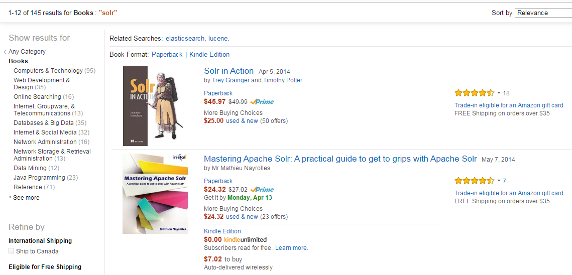
If you’re reading this blog post, you’re probably already familiar with the Facet concept in Solr. A facet is a way to count or aggregate how many elements are available for a given category. Facets also allow users to drill down and refine their searches. One common use of facets is for online stores.

Here’s a facet example for books with the word “Solr” in them, taken from Amazon.

2015-04-09_1428

To understand how Solr does it, go on the command line and fire up the techproduct example from Solr 5 by executing the following command:

pathToSolr/bin/solr -e techproducts

If you’re curious to know where the source data are located for the techproducts database, go to the folder pathToSolr/example/exampledocs/*.xml

Here’s an example of a document that’s added to the techproduct database.

Notice the cat and manu field names. We will be using them in the creation of facet.

<add><doc>
<field name="id">MA147LL/A</field>
 <field name="name">Apple 60 GB iPod with Video Playback Black</field>
 <field name="manu">Apple Computer Inc.</field>
 <!-- Join -->
 <field name="manu_id_s">apple</field>
 <field name="cat">electronics</field>
 <field name="cat">music</field>
 <field name="features">iTunes, Podcasts, Audiobooks</field>
 <field name="features">Stores up to 15,000 songs, 25,000 photos, or 150 hours of video</field>
 <field name="features">2.5-inch, 320x240 color TFT LCD display with LED backlight</field>
 <field name="features">Up to 20 hours of battery life</field>
 <field name="features">Plays AAC, MP3, WAV, AIFF, Audible, Apple Lossless, H.264 video</field>
 <field name="features">Notes, Calendar, Phone book, Hold button, Date display, Photo wallet, Built-in games, JPEG photo playback, Upgradeable firmware, USB 2.0 compatibility, Playback speed control, Rechargeable capability, Battery level indication</field>
 <field name="includes">earbud headphones, USB cable</field>
 <field name="weight">5.5</field>
 <field name="price">399.00</field>
 <field name="popularity">10</field>
 <field name="inStock">true</field>
 <!-- Dodge City store -->
 <field name="store">37.7752,-100.0232</field>
 <field name="manufacturedate_dt">2005-10-12T08:00:00Z</field>
</doc></add>

Open the following link in your favorite browser:

http://localhost:8983/solr/techproducts/select?q=*%3A*&rows=0&wt=json&indent=true&facet=true&facet.field=manu

Notice the 2 parameters:

  • facet=true
  • facet.field=manu

If everything worked as planned, you should get an answer that looks like the one below. You should see the results show how many elements are included for each manufacturer.

…
"response":{"numFound":32,"start":0,"docs":[]
 },
 "facet_counts":{
   "facet_queries":{},
   "facet_fields":{
     "manu":[
       "inc",8,
       "apache",2,
       "bank",2,
       "belkin",2,
…

Facet Pivot

Pivots are sometimes also called decision trees. Pivot allows you to quickly summarize and analyze large amounts of data in lists, independent of the original data layout stored in Solr.

One real-world example is the requirement of showing the university in the provinces and the number of classes offered in both provinces and university. Until facet pivot, it was not possible to accomplish this task without changing the structure of the Solr data.

With Solr, you drive the pivot by using the facet.pivot parameter with a comma separated field list.

The example below shows the count for each category (cat) under each manufacturer (manu).

http://localhost:8983/solr/techproducts/select?q=*%3A*&rows=0&wt=json&indent=true&facet=true&facet.pivot=manu,cat

Notice the fields:

  • facet=true
  • facet.pivot=manu,cat
"facet_pivot":{
     "manu,cat":[{
         "field":"manu",
         "value":"inc",
         "count":8,
         "pivot":[{
             "field":"cat",
             "value":"electronics",
             "count":7},
           {
             "field":"cat",
             "value":"memory",
             "count":3},
           {
             "field":"cat",
             "value":"camera",
             "count":1},
           {
             "field":"cat",
             "value":"copier",
             "count":1},
           {
             "field":"cat",
             "value":"electronics and computer1",
             "count":1},
           {
             "field":"cat",
             "value":"graphics card",
             "count":1},
           {
             "field":"cat",
             "value":"multifunction printer",
             "count":1},
           {
             "field":"cat",
             "value":"music",
             "count":1},
           {
             "field":"cat",
             "value":"printer",
             "count":1},
           {
             "field":"cat",
             "value":"scanner",
             "count":1}]},

Stats Component

The Stats Component has been around for some time (since Solr 1.4). It’s a great tool to return simple math functions, such as sum, average, standard deviation, and so on for an indexed numeric field.

Here is an example of how to use the Stats Component on the field price with the techproducts sample database. Notice the parameters:

http://localhost:8983/solr/techproducts/select?q=*:*&wt=json&stats=true&stats.field=price&rows=0&indent=true

  • stats=true
  • stats.field=price
...

"response":{"numFound":32,"start":0,"docs":[]
 },
 "stats":{
   "stats_fields":{
     "price":{
       "min":0.0,
       "max":2199.0,
       "count":16,
       "missing":16,
       "sum":5251.270030975342,
       "sumOfSquares":6038619.175900028,
       "mean":328.20437693595886,
       "stddev":536.3536996709846,
       "facets":{}}}}}

...

Mixing Stats Component and Facets

Now that you’re aware of what the stats module can do, wouldn’t it be nice if you could mix and match the Stats Component with Facets? To continue from our previous example, if you wanted to know the average price for an item sold by a given manufacturer, this is what the query would look like:

http://localhost:8983/solr/techproducts/select?q=*:*&wt=json&stats=true&stats.field=price&stats.facet=manu&rows=0&indent=true

Notice the parameters:

  • stats=true
  • stats.field=price
  • stats.facet=manu
…
"stats_fields":{
     "price":{
       "min":0.0,
       "max":2199.0,
       "count":16,
       "missing":16,
       "sum":5251.270030975342,
       "sumOfSquares":6038619.175900028,
       "mean":328.20437693595886,
       "stddev":536.3536996709846,
       "facets":{
         "manu":{
           "canon":{
             "min":179.99000549316406,
             "max":329.95001220703125,
             ...
             "stddev":106.03773765415568,
             "facets":{}},

"belkin":{
             "min":11.5,
             "max":19.950000762939453,
             ...
             "stddev":5.975052840505987,
             "facets":{}}

…

The problem with putting the facet inside the Stats Component is that the Stats Component will always return every term from the stats.facet field without being able to support simple functions, such as facet.limit and facet.sort. There’s also a lot of problems with multivalued facet fields or non-string facet fields.

Solr 5 Brings Stats to Facet

One of Solr 5’s new features is to bring the stats.fields under a Facet Pivot. This is a great thing because you can now leverage the power of the code already done for facets, such as ordering and filtering. Then you can just delegate the computing for the math function tasks, such as min, max, and standard deviation, to the Stats Component.

http://localhost:8983/solr/techproducts/select?q=*:*&wt=json&indent=true&rows=0&facet=true&stats=true&stats.field={!tag=t1}price&facet.pivot={!stats=t1}manu

Notice the parameters:

  • facet=true
  • stats=true
  • stats.field={!tag=t1}price
  • facet.pivot={!stats=t1}manu
...

"facet_counts":{
   "facet_queries":{},
   "facet_fields":{},
   "facet_dates":{},
   "facet_ranges":{},
   "facet_intervals":{},
   "facet_pivot":{
     "manu":[{
         "field":"manu",
         "value":"inc",
         "count":8,
         "stats":{
           "stats_fields":{
             "price":{
               "min":74.98999786376953,
               "max":2199.0,
...
               "sumOfSquares":5406265.926629987,
               "mean":549.697146824428,
               "stddev":740.6188014133371,
               "facets":{}}}}},
       {

...

The expression {!tag=t1} and the {!stats=t1} are named “Local Parameters in Queries”. To specify a local parameter, you need to follow these steps:

  1. Begin with {!
  2. Insert any number of key=value pairs separated by whitespace.
  3. End with } and immediately follow with the query argument.

In the example above, I refer to the stats field instance by referring to arbitrarily named tag that I created, i.e., t1.

You can also have multiple facet levels by using facet.pivot and passing comma separated fields, and the stats will be computed for the child Facet.

For example : facet.pivot={!stats=t1}manu,cat

http://localhost:8983/solr/techproducts/select?q=*:*&wt=json&indent=true&rows=0&facet=true&stats=true&stats.field={!tag=t1}price&facet.pivot={!stats=t1}manu,cat

...

"facet_pivot":{
     "manu,cat":[{
         "field":"manu",
         "value":"inc",
         "count":8,
         "pivot":[{
             "field":"cat",
             "value":"electronics",
             "count":7,
             "stats":{
               "stats_fields":{
                 "price":{
                   "min":74.98999786376953,
                   "max":479.95001220703125,
...
                   "stddev":153.31712383138424,
                   "facets":{}}}}},
           {

...

You can also mix and match overlapping sets, and you will get the computed facet.pivot hierarchies.

http://localhost:8983/solr/techproducts/select?q=*:*&wt=json&indent=true&rows=0&facet=true&stats=true&stats.field={!tag=t1,t2}price&facet.pivot={!stats=t1}cat,inStock&facet.pivot={!stats=t2}manu,inStock

Notice the parameters:

  • stats.field={!tag=t1,t2}price
  • facet.pivot={!stats=t1}cat,inStock
  • facet.pivot={!stats=t2}manu,inStock

This section represents a sample of the following sequence: facet.pivot={!stats=t1}cat,inStock

 "facet_pivot":{
     "cat,inStock":[{
         "field":"cat",
         "value":"electronics",
         "count":12,
         "pivot":[{
             "field":"inStock",
             "value":true,
             "count":8,
             "stats":{
               "stats_fields":{
                 "price":{
                   "min":74.98999786376953,
                   "max":399.0,
             ...
                   "facets":{}}}}},
           {
             "field":"inStock",
             "value":false,
             "count":4,
             "stats":{
               "stats_fields":{
                 "price":{
                   "min":11.5,
                   "max":649.989990234375,
...
                   "facets":{}}}}}],
         "stats":{
           "stats_fields":{
             "price":{
               "min":11.5,
               "max":649.989990234375,
...
               "facets":{}}}}},

This section represents a sample of the following sequence:

facet.pivot={!stats=t2}manu,inStock

It’s the sequence that was produced by the query shown in the URL above.

 "facet_pivot":{
     "cat,inStock":[{
         "field":"cat",
         "value":"electronics",
         "count":12,
         "pivot":[{
             "field":"inStock",
             "value":true,
             "count":8,
             "stats":{
               "stats_fields":{
                 "price":{
                   "min":74.98999786376953,
                   "max":399.0,
             ...
                   "facets":{}}}}},
           {
             "field":"inStock",
             "value":false,
             "count":4,
             "stats":{
               "stats_fields":{
                 "price":{
                   "min":11.5,
                   "max":649.989990234375,
...
                   "facets":{}}}}}],
         "stats":{
           "stats_fields":{
             "price":{
               "min":11.5,
               "max":649.989990234375,
...
               "facets":{}}}}},

How about Solr Cloud?

With Solr 5, it’s now possible to compute fields stats for each pivot facet constraint in a distributed environment, such as Solr Cloud. A lot of hard work went into solving this very complex problem. Getting the results from each shard and quickly and effectively merging them required a lot refactoring and optimization. Each level of facet pivots needs to be analyzed and will influence that level’s children facets. There is a refinement process that iteratively selects and rejects items at each facet level when results are coming in from all the different shards.

Does Pivot Faceting Scale Well?

Like I mentioned above, Pivot Faceting can be expensive in a distributed environment. I would be careful and properly set appropriate facet.list parameters at each facet pivot level. If you’re not careful, the number of dimensions requested can grow exponentially. Having too many dimensions can and will eat up all the system resources.  The online documentation is referring to multimillions of documents spread across multiple shards getting sub-millisecond response times for complex queries.

Conclusion

This tutorial should have given you a solid foundation to get you started on slicing and dicing your data. I have defined the concepts Pivot Facet, Stats Module, and Local Parameter. I also have shown you query examples using those concepts and their results. You should now be able to go out on your own and build your own solution. You can also give us a call if you need help. We provide training and consulting services that will get you up and running in no time.

Do you have any experience building analytical systems with Solr? Please share your experience below.

In this tutorial, I will show you how to run Solr as a Microsoft Windows service. Up to version 5.0.0, it was possible to run Solr inside the Java web application container of your choice. However, since the release of version 5.0.0, the Solr team at Apache no longer releases the solr.war file. This file was necessary to run Solr from a different web application container such as Tomcat. Starting with version 5.0.0, Solr will be distributed only as a self-contained web application, using an embedded version of Jetty as a container.

Unfortunately, Jetty does not have a nice utility like Tomcat’s to register itself as a service on Microsoft Windows. I had to research and experiment to come up with a clean and easily-reproduced solution. I tried to follow the Jetty website instructions and adapt them to make Jetty work with Solr, but I was not able to stop the service cleanly. When I would request a “stop” from the Windows Service Manager, the service was flip-flopping between “starting” and “stopping” statuses. Then I discovered a simple tool, NSSM, that did exactly what I wanted. I will be using the NSSM tool in this tutorial.

Applications to Download

File System Setup

Taking Solr 5.0.0 as an example, first, extract Solr and NSSM to the following path on your file system (adapt paths as necessary).

C:\Program Files\solr-5.0.0
C:\Program Files\nssm

Setting up Solr as a service

On the command line, type the following:

"c:\Program Files\nssm\win64\nssm" install solr5

Fill out the path to the solr.cmd script, and the startup directory should be filled in automatically. Don’t forget to input the -f (foreground) parameter so that NSSM can kill it when it needs to be stopped or restarted.

Application tab on NSSM Service Editor screen capture to show path to Solr start script

The following step is optional, but I prefer having a clean and descriptive name in my Windows Service Manager. Under the details tab, fill out the Display name and Description.

Details tab for NSSM service installer for setting up Solr 5 as a service on Microsoft Windows

Click on Install service.

NSSM confirmation box saying "Solr5" installed successfully

Check that the service is running.

Microsoft Windows Component Services Running Solr 5

Go to your favorite web browser and make sure Solr is up and running.

Solr 5 running as a service on Microsoft Windows

Conclusion

I spent a few hours finding this simple solution, and I hope this tutorial will help you set up Solr as a Microsoft Windows service in no time. I invite you to view the solr.cmd file content to find the parameters that will help you customize your Solr setup. For instance, while looking inside this file, I realized there I needed to add the -f parameter to run Solr in the foreground. That was key to get it running the way I needed it.

If you successfully used a different approach to register Solr 5 as a service, please share it in the comments section below.

Responsive DesignAs a Search Expert at Norconex, I am often assigned the task of integrating web accessibility standards within a search user interface for our customers in the government sector; these customers look to web accessibility to improve the overall search experience of their current enterprise’s search offering. And, of course, we have noticed a growing trend in the desire for search user interfaces that can respond to various screen sizes on various devices.

This post will look at the strategies I have used to design a web accessible search user interface and present why it is equally important to tackle a responsive web design.  To illustrate an accessible response web design, I will demonstrate the Elections.ca website project that I have recently worked on with the Google Search Appliance (GSA). (more…)

Over the past few years we’ve seen a drastic improvement in search interfaces.  The development of ugly search boxes and incomprehensible search result screens should now (hopefully) be a thing of the past.  New search UI’s are designed and developed daily, that are crisp, clean, well thought out, and really help guide users to the information they’re looking for.  Search based concepts and technologies are finally starting to be properly recognized as being as important as the content they’re put in place to help discover.  A clean, well thought out search user interface not only makes a large difference in helping users navigate site information, but also goes a long ways towards bringing users back for more. (more…)